How to Draw Phase Planes Matlab
For any differential equation in normal form
\[ y' = f(x,y) \qquad \mbox{or} \qquad \frac{{\text d}y}{{\text d}x} = f(x,y) \]
where f(10,y) is a well defined in some domain slope function, it is possible to obtain a graphical information about general beliefs of the solution curves (call trajectories) from the differential equation itself without bodily solution formula.
In the previous section, we bear witness that direction fields or slope fields are very important features of differential equations because they provide a qualitative behavior of solutions. Notwithstanding, more precise information results from including in the plot some typical solution curves or trajectories.
A plot that shows representative sample of trajectories for a given starting time order differential equation is called stage portrait.
This department shows how to include sample trajectories into tangent field to obtain a stage portrait for a given differential equation.
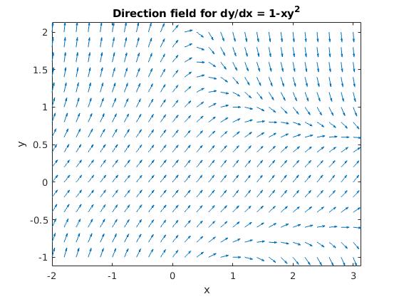
The main matlab command for plotting direction fields is quiver, used in conjuction with meshgrid. To plot the gradient field of a differential equation \( y' = f(10,y) \) on the rectangle 𝑎 ≤ ten ≤ b, c ≤ y ≤ d, type the following sequence of commands:
The first command sets upward a 26 by 16 grid of uniformly spaced points in the rectangular domain [-two,3] × [-1,2]. The second control evaluates the right-hand side of the differential equation \( y' = ane- x\,y^2 \) at the filigree points, thereby producing the slopes, southward = f(x,y), at these points. The vectors (ane,s) have the desired slopes just have different lengths at the unlike filigree points. The quiver command, used for plotting vector fields, requires iv inputs: the array x of x-values, the array y of y-values, and arrays consisting of the two components of the management field vectors. Since all of these arrays must have the same size, the code ones(size(southward)) conveniently creates an array of ones of the same size as s. In the last command, axis tight eliminates white infinite at the edges of the direction field. The outcome looks similar this:
While this film is correct, it is somewhat hard to read considering of the fact that many of the vectors are quite small. You can go a better picture by rescaling the arrows so that they do not vary in magnitude---for example, past dividing each vector (1,due south) by its length \( \| (1,southward)\| = \sqrt{1 + s^2} . \) In order to achieve it in matlab, nosotros alter the preceeding sequence of commands to:
 | The fifth entry, 0.5, in the quiver command reduces the length of the vectors past half and prevents the arrow heads from swallowing upwardly the tails of nearby vectors. The result is presented at the left. The picture strongly suggests that some solutions approach a specific curve, simply others tend to minus infinity. This specific bend is called the separatrix. |
Unless the special purposed field program is used, plotting slope fields in matlab requiries a bit of work. The post-obit programme utilizes the born control quiver(x,y,dx,dy) that plots an due north × n array of vectors with x- and y- components specified by the northward×n matrices dx and dy, based at the xy-points in the plane whose x- and y-coordinates are specified by the n×n matrices x and y.
Another Octave lawmaking:
Another lawmaking with numerical solution
% portrait.k [10,y] = meshgrid(-three:0.2:3,-3:0.2:iii); n = size(x); u = ones(n); v = one - x.*y.^2; for i = 1:numel(x) rac = two*sqrt(u(i)^two + v(i)^2); u(i) = u(i)/rac; v(i) = five(i)/rac; end xspan = [-two,iii]; x0 = -2; [twenty,yy] = ode45(@(x,y) 1-x*y^2, xspan, x0); effigy concur on quiver(x,y,u,5) plot(xx,yy,'-') We use Chebfun to plot phase portrait:
??????
Fault using chebop/solveivp (line 240) The number of initial/final conditions does non match the differential order(s) appearing in the problem. Error in \ (line 49) [varargout{one:nargout}] = solveivp(N, rhs, pref, varargin{:});
| | |

To plot direction fileds along with some solutions, use the control streamline
% define arrays x, y, u, and v: [ten,y] = meshgrid(0:0.one:one,0:0.1:1); u = x; v = -y; % Create a quiver plot of the data. Plot streamlines that start at different points along the line y=one. figure quiver(x,y,u,v) startx = 0.1:0.1:1; starty = ones(size(startx)); streamline(x,y,u,v,startx,starty) The best fashion to plot direction fields is to use existing m-files, credited to John Polking from Rice University (http://math.rice.edu/~polking/). He is the author of two special matlab routines: dfield8 plots direction fields for single, beginning lodge ordinary differential equations, and allows the user to plot solution curves; pplane8 plots vector fields for planar democratic systems. It allows the user to plot solution curves in the phase plane, and it too enables a variety of time plots of the solution. Information technology will also find equilibrium points and plot separatrices. The latest versions of dfield8 and pplane8 m-functions are not compatible with the latest matlab version. Y'all tin can grab its modification that works from dfield.1000
Since matlab has no friendly subroutine to plot direction fields for ODEs, we present several codes that allow to plot these fields directly. Many others can establish on the Internet. The following Octave code shows how to plot the direction field for the linear differential equation \( y' = v\,y - 3\,10 . \)
The following lawmaking presents the function version to plot management field for first gild ODE y' = f(t,y)
% plot direction field for offset order ODE y' = f(t,y) part dirfield f = @(t,y) -y^2+t % f = @(independent_var, dependent_var) % mathematical expression y in terms of t figure; dirplotter(f, -1:.2:3, -2:.ii:ii) % dirfield(f, t_min:t_spacing:t_max, y_min:y_spacing:y_min) % using t-values from t_min to t_max with spacing of t_spacing % using y-values from y_min to t_max with spacing of y_spacing end Some other function:
part dirplotter(f,tval,yval) % plots management field using aboved defined (f,tval,yval) [tm,ym]=meshgrid(tval,yval); % creates a grid of points stored in matrices in the (t,y)-aeroplane dt = tval(2) - tval(1); % determines t_spacing and y_spacing based on tval dy = yval(ii) - yval(1); % determines t_spacing and y_spacing based on yval fv = vectorize(f); % prevents matrix algebra; if f is a function handle fv is a string if isa(f,'function_handle') % if f is part handle fv = eval(fv); % plough fv into a part handle from a string end yp=feval(fv,tm,ym); % evaluates differential equation fv from tm and ym from meshgrid s = 1./max(1/dt,abs(yp)./dy)*0.35; h = ishold; % define h every bit ishold which returns one if hold is on, and 0 if information technology is off quiver(tval,yval,s,s.*yp,0,'.r'); hold on; % plots vectors at each indicate w management based on righthand side of differential equation quiver(tval,yval,-s,-due south.*yp,0,'.r'); if h % h above defined every bit ishold hold on % retain electric current plot else % refers to all non h concord off % resets axes properties to default end axis([tval(1)-dt/2,tval(end)+dt/ii,yval(ane)-dy/2,yval(end)+dy/2]) % sets the scaling for axes on electric current graph to ends of tval and yval end % Elementary direction field plotter clear; [T Y]=meshgrid(-2:0.2:2,-2:0.two:2); dY=cos(iii*T)+Y./T; dT=ones(size(dY)); calibration=sqrt(1+dY.^two); figure; quiver(T, Y, dT./scale, dY./scale,.5,'Color',[1 0 0]); xlabel('t'); ylabel('y'); championship('Direction Field for dy/dt'); axis tight; hold on; % change color % do multiple examples, ten.^2-y.^two; use T, etc % Uncomplicated management field plotter clear; [T Y]=meshgrid(-2:0.2:ii,-2:0.2:two); dY=T.^2-Y.^2; dT=ones(size(dY)); scale=sqrt(1+dY.^2); figure; quiver(T, Y, dT./scale, dY./scale,.five,'Colour',[0 1 0]); xlabel('t'); ylabel('y'); title('Direction Field for dy/dt'); axis tight; concord on; Example: **DESCRIPTION OF Problem GOES HERE** This is a description for some MATLAB code. MATLAB is an extremely useful tool for many different areas in engineering, applied mathematics, information science, biology, chemistry, and so much more. It is quite amazing at treatment matrices, but has lots of contest with other programs such every bit Mathematica and Maple. Here is a code snippet plotting two lines (y vs. x and z vs. ten) on the same graph. Click to view the code!
figure(ane) plot(x, y, 'Color', [1 0 0]) %blue line concord on plot(x, z, 'Colour', [0 1 0]) %greenish line - Trefethen, Fifty.Northward., Birkisson, A., Driscoll, T.A., Exploring ODEs, SIAM, Philadelphia, 2018.
Source: https://www.cfm.brown.edu/people/dobrush/am33/Matlab/ch2/phase.html
0 Response to "How to Draw Phase Planes Matlab"
Postar um comentário